Note
Go to the end to download the full example code.
Happy individual
In Four Ways of Thinking our friends switch focus.

The specific question we look at here is this: Imagine, after you have paid your bills, you have more than $200 per month to spend divided between three categories: (1) material items, (2) experiences and (3) time-saving services. How should you spend this money in order to be as happy as possible? We try to answer this question using a questionnaire conducted by Whillans et al. (2017). We look in particular at 1067 people with varying incomes, but all with a budget of at least $200 to spend. The study participants typically spent about $250 on (each of) material items and experiences, and about half as much on time-saving.
All the participants were asked the question:
Please imagine a ladder with steps numbered from zero at the bottom to ten at the top.
Suppose we say that the top of the ladder represents the best possible life for you
and the bottom of the ladder represents the worst possible life for you.
On which step of the ladder would you say you personally feel you stand at this time?
This is how see Whillans et al. measure happiness in the study I write about in the book. In this section we dig in to the data of the replies they received in one of the studies they conducted as part of their work.
Loading in the data
import numpy as np
import pandas as pd
import matplotlib.pyplot as plt
import statsmodels.api as sm
import statsmodels.formula.api as smf
import random

from pylab import rcParams
rcParams['figure.figsize'] = 12/2.54, 12/2.54


# Find people who spent more than 200 dollars in total
# These are the people we will look at in this study.

# The data file we use here is a adapted from the data from here https://osf.io/vr9pa/
# Study 7 US Qualtrics data.
df=pd.read_csv('../data/spending.csv')

morethan200=df['spent_on_MATA']+df['spent_on_TSA']+df['spent_on_EXPA'] >200
df=df[morethan200]

print('The average happiness score was %.2f.' % np.mean(df['Happiness']))
print('The standard deviation in happiness score was %.2f.' %np.std(df['Happiness']))
print('90 percent of people had a happiness score of %.2f or more.' % np.quantile(df['Happiness'],0.9))
print('10 percent of people had a happiness score of %.2f or less.' % np.quantile(df['Happiness'],0.1))
The average happiness score was 7.15.
The standard deviation in happiness score was 1.84.
90 percent of people had a happiness score of 10.00 or more.
10 percent of people had a happiness score of 5.00 or less.
Try it yourself!
Think about the answer you would give to this question now. By putting yourself in the participants shoes you can better understand what it means when people rank their happiness.
The participants gave a wide-range of answers, with an average of 7.15, but scores as low as 3 and as high as 10 were not untypical.
Spending money on saving time
Let’s start by looking at the difference in average happiness. Are people who spend money on saving time happier?
didspend=df['spent_on_TSA']>0
didntspend=df['spent_on_TSA']<=0
mean_did= np.mean(df['Happiness'][didspend])
mean_didnt= np.mean(df['Happiness'][didntspend])

print('The average happiness score for those who spent on time-saving was %.2f.' % mean_did)
print('The average happiness score for those who did not spent on time-saving was %.2f.' % mean_didnt)

std_did=np.nanstd(df['Happiness'][didspend])
n_did=len(df['Happiness'][didspend])
std_didnt=np.nanstd(df['Happiness'][didntspend])
n_didnt=len(df['Happiness'][didntspend])
cohensd=(mean_did-mean_didnt)/np.sqrt(((n_did-1)*std_did**2+(n_didnt-1)*std_didnt**2)/(n_did+n_didnt-2))

print('The Cohens D for this difference is %.2f' % cohensd)
The average happiness score for those who spent on time-saving was 7.43.
The average happiness score for those who did not spent on time-saving was 6.63.
The Cohens D for this difference is 0.44
Cohen’s D is a statistic for measuring effect size. How big an effect does spending on time saving have? An effect of 0.44 is considered to be medium.
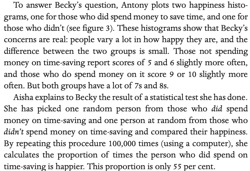
The difference between the two groups can’t be attributed to chance, since over one thousand people were surveyed, but it is not a particularly large difference. But it is not particularly large. This point is illustrated below in a histogram for those who did spend money on time saving (top in the figure below) and those who did not (bottom in the figure below).
def FormatFigure(ax):
    ax.legend(loc='upper left')
    ax.set_ylim(0,0.32)
    ax.spines['top'].set_visible(False)
    ax.spines['right'].set_visible(False)
    ax.set_ylabel('')
    ax.set_xlabel('Average Happiness (0-10)')
    ax.set_ylabel('Proportion of people')
    ax.set_xticks(np.arange(0,11,step=1))


fig,(ax1,ax2)=plt.subplots(2,1)
ax1.hist(df['Happiness'][didspend], np.arange(0.01,10.5,1), color='orange', edgecolor = 'black',linestyle='-',alpha=0.5, label='Spent on saving time', density=True,align='right')
FormatFigure(ax1)
ax2.hist(df['Happiness'][didntspend], np.arange(0.01,10.5,1), alpha=0.5, edgecolor = 'black', label='Did not spend on saving time',  density=True,align='right')
FormatFigure(ax2)

plt.show()

What is most striking is how little these two histograms differ, with those not spending money of time-saving shifted very slightly to the left. There are more tens in the did spend group, but otherwise they are not that different.
In the code below we pick pairs of people at random - one from thosee who did spend on time-saving and one person who didn’t spend on time-saving. We then look at the proportion of times the one who did spend on time-saving is happier.
df_did=df['Happiness'][didspend]
df_didnt=df['Happiness'][didntspend]
rand_did=df_did.sample(10000,replace=True)
rand_didnt=df_didnt.sample(10000,replace=True)
print('The person who did spend on time-saving is happiest %.2f percent of times.' % (np.mean(np.array(rand_did)>np.array(rand_didnt))*100))
The person who did spend on time-saving is happiest 55.12 percent of times.
If you currently do not spend any of your budget on time-saving, then this value of around 55% gives an estimate of the probability you would be happier if you did. Likewise, if you currently do spend some of your budget on time-saving, then the probability you would be happier if you didn’t make the spend is 45%.
In the book I let the friends explain:
It thus makes sense to spend money on time-saving, but results are by no means guaranteed.
What to spend money on
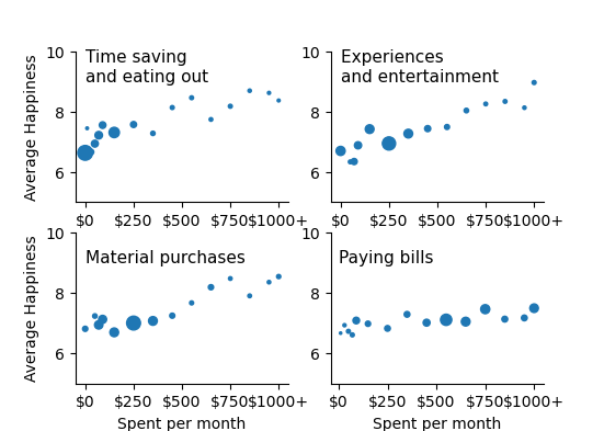
How much happier can we expect to be per dollar spent on, respectively, material items, experiences and time-saving?
To answer this question, we plot average happiness against the amount of money people spent.
# The data is coded for different spending levels.
# This converts the spending levels in to dollars.
scale_spending = np.array([0] + list(range(10,100,20)) + list(range(150,1000,100)) + [1000] + [1000])
scale_spending = np.append(scale_spending, [np.nan,np.nan,np.nan])
scale_spending_labels = {0.0: '$0',
 1.0: '$1-$19',
 2.0: '$20-$39',
 3.0: '$40-$59',
 4.0: '$60-$79',
 5.0: '$80-$99',
 6.0: '$100-$199',
 7.0: '$200-$299',
 8.0: '$300-$399',
 9.0: '$400-$499',
 10.0: '$500-$599',
 11.0: '$600-$699',
 12.0: '$700-$799',
 13.0: '$800-$899',
 14.0: '$900-$999',
 15.0: '$1000-$2500',
 16.0: 'More than $2500'}

rcParams['figure.figsize'] = 14/2.54, 10/2.54

fig,axs=plt.subplots(2,2)

for i,original_name in enumerate(['MATA','EXPA','TSA','Bills']):

    mean_happy = np.zeros(len(scale_spending))*np.nan
    std_happy = np.zeros(len(scale_spending))*np.nan
    num_value = np.zeros(len(scale_spending))*np.nan

    #Measure happiness for each
    for j,lb in enumerate(np.unique(scale_spending)):
        dfs=df[df['spent_on_' + original_name]==lb]
        num_value[j]=len(dfs)
        if len(dfs)>5:
            mean_happy[j]=np.nanmean(dfs['Happiness'])
            std_happy[j]=np.nanstd(dfs['Happiness'])/np.sqrt(len(dfs))

    ax=axs[int(np.ceil(i/2))-1][np.remainder(i,2)]

    #Plot the graph.
    ax.scatter(scale_spending, mean_happy,s=(num_value/4)+1)
    print(mean_happy)

    ax.set_ylim(5,10)
    ax.spines['top'].set_visible(False)
    ax.spines['right'].set_visible(False)
    if i==0:
        ax.text(0,9,'Material purchases', fontsize=11)
        ax.set_ylabel('Average Happiness')
        ax.set_xlabel('Spent per month')
    if i==1:
        ax.text(0,9,'Experiences \nand entertainment', fontsize=11)
    if i==2:
        ax.text(0,9,'Time saving \nand eating out', fontsize=11)
        ax.set_ylabel('Average Happiness')
    if i==3:
        ax.text(0,9,'Paying bills', fontsize=11)
        ax.set_xlabel('Spent per month')
    ax.set_xticks(np.arange(0,1100,step=250))
    ax.set_xticklabels(['$0','$250','$500','$750','$1000+'])

plt.show()
[6.80952381        nan        nan 7.23333333 6.93913043 7.12264151
 6.69291339 7.         7.07086614 7.24390244 7.66666667 8.18604651
 8.47368421 7.9        8.35294118 8.53846154        nan        nan
        nan        nan]
[6.69565217        nan        nan 6.33333333 6.3442623  6.88095238
 7.41732283 6.94217687 7.26771654 7.43333333 7.48717949 8.03125
 8.25       8.33333333 8.125      8.95833333        nan        nan
        nan        nan]
[6.63172043 7.44444444 6.66       6.93589744 7.21505376 7.54929577
 7.30555556 7.56896552 7.27586207 8.13043478 8.45454545 7.73684211
 8.17391304 8.6875     8.61538462 8.36363636        nan        nan
        nan        nan]
[       nan 6.66666667 6.92857143 6.72727273 6.60869565 7.08450704
 6.97727273 6.82352941 7.28846154 7.01282051 7.10798122 7.04724409
 7.45985401 7.12962963 7.16981132 7.49180328        nan        nan
        nan        nan]
We see that those with the most money to spend are the happiest. Those with expenditure of $1000 per month on each of material, experiences and time-saving have a happiness of around 8.5 on average. Paying bills does not make people happier.
We would all love to have $1000 to spend on each of the three categories, but what is the best investment on a limited budget?
Here it is important to notice that time-saving initially increases faster per dollar spent than the lines for material purchases or experiences. We can estimate how more rapid this increase is using linear regression, which measures the steepness of the increase for each factor.
model_fit=smf.ols(formula='Happiness' + ' ~  spent_on_MATA + spent_on_TSA + spent_on_EXPA + spent_on_Bills' , data=df).fit()
print(model_fit.summary())

print('For every $100 spent per month on time saving, %.2f points of happiness gained' % (100.0*model_fit.params['spent_on_TSA']))
print('For every $100 spent per month on experiences, %.2f points of happiness gained' % (100.0*model_fit.params['spent_on_EXPA']))
print('For every $100 spent per month on material purchases, %.2f points of happiness gained' % (100.0*model_fit.params['spent_on_MATA']))
                            OLS Regression Results
==============================================================================
Dep. Variable:              Happiness   R-squared:                       0.098
Model:                            OLS   Adj. R-squared:                  0.094
Method:                 Least Squares   F-statistic:                     28.73
Date:                Tue, 03 Sep 2024   Prob (F-statistic):           1.08e-22
Time:                        07:11:26   Log-Likelihood:                -2107.6
No. Observations:                1067   AIC:                             4225.
Df Residuals:                    1062   BIC:                             4250.
Df Model:                           4
Covariance Type:            nonrobust
==================================================================================
                     coef    std err          t      P>|t|      [0.025      0.975]
----------------------------------------------------------------------------------
Intercept          6.4082      0.128     49.897      0.000       6.156       6.660
spent_on_MATA      0.0007      0.000      2.840      0.005       0.000       0.001
spent_on_TSA       0.0013      0.000      4.630      0.000       0.001       0.002
spent_on_EXPA      0.0011      0.000      4.154      0.000       0.001       0.002
spent_on_Bills  9.137e-05      0.000      0.482      0.630      -0.000       0.000
==============================================================================
Omnibus:                       33.304   Durbin-Watson:                   1.959
Prob(Omnibus):                  0.000   Jarque-Bera (JB):               35.612
Skew:                          -0.438   Prob(JB):                     1.85e-08
Kurtosis:                       3.180   Cond. No.                     1.86e+03
==============================================================================

Notes:
[1] Standard Errors assume that the covariance matrix of the errors is correctly specified.
[2] The condition number is large, 1.86e+03. This might indicate that there are
strong multicollinearity or other numerical problems.
For every $100 spent per month on time saving, 0.13 points of happiness gained
For every $100 spent per month on experiences, 0.11 points of happiness gained
For every $100 spent per month on material purchases, 0.07 points of happiness gained
This method tells us that for every $100 spent in different ways how much happiness is gained. So, increasing spending from $0 per month to around $500 per month on saving time (if you have that money to spare) would make you almost 0.13*5 = 0.65 point (on a scale of 0 to 10) happier.
In the book I write that “[Antony] finds that every $100 spent on time-saving leads to an average gain of 0.31 points on the happiness scale. So, increasing spending from $0 per month to around $300 per month on saving time provides almost one extra point of happiness. “
This claim is based on a regression model that includes a non-linear term to capture the saturation at high levels of spending. I repeat the regression with squared terms as follows.
for original_name in ['MATA','Bills','TSA','EXPA']:
    variable_of_interest='spent_on_' + original_name
    df[variable_of_interest + '_2']=df[variable_of_interest]**2

model_fit=smf.ols(formula='Happiness' + ' ~  spent_on_MATA + spent_on_TSA + spent_on_EXPA + spent_on_MATA_2 + spent_on_TSA_2 + spent_on_EXPA_2' , data=df).fit()
print(model_fit.summary())
                            OLS Regression Results
==============================================================================
Dep. Variable:              Happiness   R-squared:                       0.104
Model:                            OLS   Adj. R-squared:                  0.099
Method:                 Least Squares   F-statistic:                     20.45
Date:                Tue, 03 Sep 2024   Prob (F-statistic):           9.73e-23
Time:                        07:11:26   Log-Likelihood:                -2104.0
No. Observations:                1067   AIC:                             4222.
Df Residuals:                    1060   BIC:                             4257.
Df Model:                           6
Covariance Type:            nonrobust
===================================================================================
                      coef    std err          t      P>|t|      [0.025      0.975]
-----------------------------------------------------------------------------------
Intercept           6.3403      0.158     40.160      0.000       6.031       6.650
spent_on_MATA       0.0006      0.001      0.757      0.449      -0.001       0.002
spent_on_TSA        0.0031      0.001      4.119      0.000       0.002       0.005
spent_on_EXPA       0.0014      0.001      2.049      0.041    5.77e-05       0.003
spent_on_MATA_2  3.042e-07   8.34e-07      0.365      0.715   -1.33e-06    1.94e-06
spent_on_TSA_2  -2.319e-06    9.1e-07     -2.549      0.011    -4.1e-06   -5.34e-07
spent_on_EXPA_2 -4.064e-07   7.71e-07     -0.527      0.598   -1.92e-06    1.11e-06
==============================================================================
Omnibus:                       35.731   Durbin-Watson:                   1.968
Prob(Omnibus):                  0.000   Jarque-Bera (JB):               38.455
Skew:                          -0.455   Prob(JB):                     4.46e-09
Kurtosis:                       3.188   Cond. No.                     1.06e+06
==============================================================================

Notes:
[1] Standard Errors assume that the covariance matrix of the errors is correctly specified.
[2] The condition number is large, 1.06e+06. This might indicate that there are
strong multicollinearity or other numerical problems.
Notice that spending time on time saving This analysis is further supported by the following graph, which looks at how happiness depends on the proportion of money spent on saving time for people who spend more than $200 per month on the three categories.
df['Prop_TS']=df['spent_on_TSA']/(df['spent_on_MATA']+df['spent_on_TSA']+df['spent_on_EXPA'] )
df['Prop_EXP']=df['spent_on_EXPA']/(df['spent_on_MATA']+df['spent_on_TSA']+df['spent_on_EXPA'] )
df['Prop_MATA']=df['spent_on_MATA']/(df['spent_on_MATA']+df['spent_on_TSA']+df['spent_on_EXPA'] )


rcParams['figure.figsize'] = 16/2.54, 10/2.54

scale_of_interest=np.append(np.arange(0,0.71,0.1), 1.0)
fig,axs=plt.subplots(1,3)

axs[0].set_ylabel('Average Happiness (0-10)')

for j,variable_of_interest in enumerate(['Prop_TS', 'Prop_EXP', 'Prop_MATA']):

    ax=axs[j]
    mean_happy = np.zeros(len(scale_of_interest)-1)
    std_happy = np.zeros(len(scale_of_interest)-1)
    num_value = np.zeros(len(scale_of_interest)-1)
    for i,lb in enumerate(scale_of_interest[:-1]):
        lbp1=scale_of_interest[i+1]
        dfs=df[np.logical_and(df[variable_of_interest]>=lb,df[variable_of_interest]<lbp1)]
        mean_happy[i]=np.mean(dfs['Happiness'])
        std_happy[i]=np.std(dfs['Happiness'])/np.sqrt(len(dfs))
        num_value[i]=len(dfs)

    ax.scatter(scale_of_interest[:-1], mean_happy,s=num_value)

    ax.spines['top'].set_visible(False)
    ax.spines['right'].set_visible(False)
    ax.set_xlim(-0.05,0.75)
    ax.set_ylim(6,9)


    ax.set_xticks(np.arange(0,0.8,step=0.2))
    ax.set_xticklabels(['0%','20%','40%','60%'  ])

    if j==2:
        ax.text(0,8.3,'Material purchases', fontsize=11)
    if j==1:
        ax.text(0,8.3,'Experiences \nand entertainment', fontsize=11)
        ax.set_xlabel('Percentage spending')

    if j==0:
        ax.text(0,8.3,'Time saving \nand eating out', fontsize=11)

plt.show()
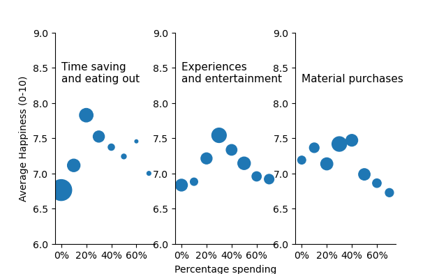
Happiness reaches a maximum at around 20% to 30% spending on time-saving and on experiences and entertainment. Using too much of your budget to buy material items leads to a decrease in happiness.
Remeber that the size of the circles are the proportion of people in that category We can calulate
print('The average person spend %.2f percent of their budget on time saving' % (100.0*np.mean(df['Prop_TS'])))
print('The average person spend %.2f percent of their budget on experiences' % (100.0*np.mean(df['Prop_EXP'])))
print('The average person spend %.2f percent of their budget on material purchases' % (100.0*np.mean(df['Prop_MATA'])))
The average person spend 17.11 percent of their budget on time saving
The average person spend 39.77 percent of their budget on experiences
The average person spend 43.12 percent of their budget on material purchases
This suggests that most of us could benefit from increasing our spending on time saving.
Summary: If you currently spend very little on money on time-saving today then investing between $100 and $300 can probably make you a fair bit happier. Spending on experiences is less effective, and spending on material purchases is not effective.
Causation
Can we say that time-saving purchases cause us to become happier? And, if so, what should I buy!?!?
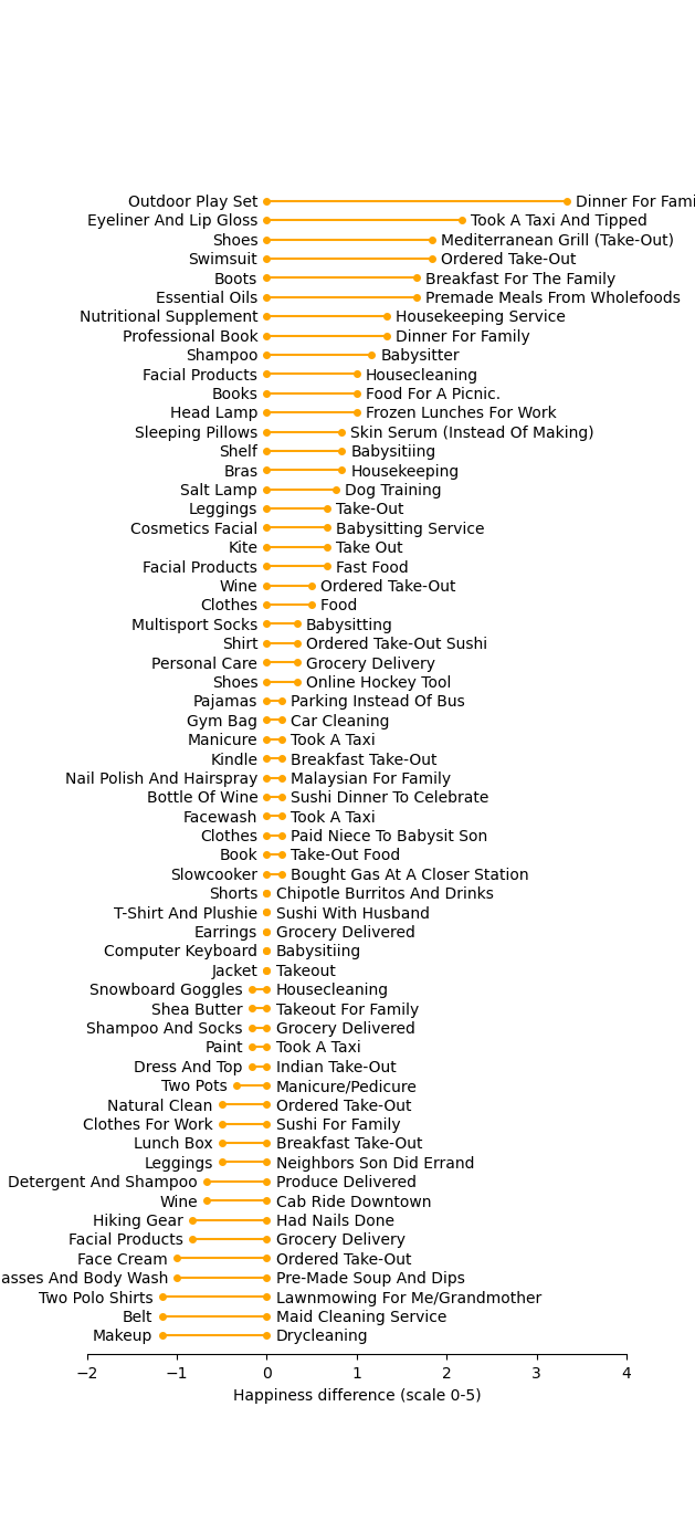
The researchers conducted an experiment to answer this question. They recruited people at a science fair, giving them $40 one week to make a time-saving purchase and $40 another week (either before or after) to make a material purchase. Below is a plot of what they bought on each occasion (material left, time-saving right) and the difference in happiness they reported each time.
For more details of the study see Whillans et al.. The data from the study can be accessed here.
rcParams['figure.figsize'] = 16/2.54, 35/2.54
fig,ax=plt.subplots(num=1)


# The data file we use here is a adapted from the data from `here <https://osf.io/vr9pa/>`_
# Study 8 Field Study data.
df=pd.read_csv("../data/happy_buy.csv",sep=';')

df['DIFF_PA']=  df['TP_PA']-df['MAT_PA']
df=df.sort_values('DIFF_PA')

i=0
for di in df.iterrows():

    i=i+1
    d=di[1]
    cl='orange'

    ax.plot([0,d['TP_PA']-d['MAT_PA']],[i,i], linestyle='solid', markersize=4, marker='o', color=cl)
    if (d['TP_PA'] > d['MAT_PA']):
        ax.text(d['TP_PA']-d['MAT_PA']+0.1,i-0.25, d['TS_Purchase'] , color='black' )
        ax.text(0-0.1,i-0.25, d['MAT_Item_1'], ha='right' , color='black')
    else:
        ax.text(d['TP_PA']-d['MAT_PA']-0.1,i-0.25, d['MAT_Item_1'], ha='right' , color='black' )
        ax.text(0+0.1,i-0.25, d['TS_Purchase'] , color='black' )

ax.set_yticks([-10,100])
ax.set_ylim(0,61)
ax.set_xlim(-2,4)
ax.spines['top'].set_visible(False)
ax.spines['right'].set_visible(False)
ax.spines['left'].set_visible(False)
ax.set_xlabel('Happiness difference (scale 0-5)')
plt.show()

np.sum(df['DIFF_PA']>0.2)
np.sum(df['DIFF_PA']<-0.2)
np.int64(14)
Answer to fourth question: Again, there are no guarantees that eating out or getting a babysitter will make you happy, but it worked for 26 out of the 60 people participating in the study, with only 14 being happier with a material purchase.
Total running time of the script: (0 minutes 1.687 seconds)